

The concluding part shifts to the forces that actively shape option prices: the Option Greeks. These mathematical sensitivities— Delta, Gamma, Theta and Vega—determine how premiums respond to changes in key variables such as movement in the underlying asset, time and changes in volatility. If the premium represents the price, the Greeks are the underlying mechanics that constantly reshape this price.
Without understanding them, options trading becomes less of a strategy and more of a gamble. By mastering the Greeks, one can move from being a hopeful speculator to a disciplined strategist.
Delta: the directional engine
Delta tells you how much an option’s price (or premium) will change when the underlying stock or index moves by Rs.1.
- Call options (profit when the underlying price rises; so you gain if price goes up): Delta ranges from 0 to 1.
- Put options (profit when the underlying price falls; so, you gain if price goes down): Delta ranges from 0 to -1.
Example:
- A call option with Delta 0.4 will gain Rs.4 if the stock rises Rs.10.
- A put option with Delta -0.5 will lose Rs.5 if the stock rises Rs.10.
Delta and moneyness
In the Money (ITM): Delta between 0.5 and 1. Strong reaction to price moves, higher chance of expiring profitable.
Risk: Though ITM options are more resilient to time decay, if the market moves against anticipated direction, losses pile up quickly.
At the Money (ATM): Delta around 0.5. Balanced—small moves can push ATM option towards profitability (ITM) or loss (OTM).
Risk: If the stock stays flat, time decay (or theta) eats away the premium.
Out of the Money (OTM): Delta between 0 and 0.5. Often cheap, but less responsive.
Risk: An OTM option with Delta 0.1 may only gain Rs.5 even if the stock jumps by Rs.50. However, time decay (or theta) can wipe out such small gain.
Another way to interpret Delta is as a rough probability of finishing profitable:
- Delta 0.2 means around 20% chance of expiring profitable.
- Delta 0.6 means around 60% chance of expiring profitable.
So, while OTM options look attractive because of low premiums, their low Delta means the odds of success are small. ITM options may cost more, but their higher Delta signals a much better chance of profit.
How option prices change
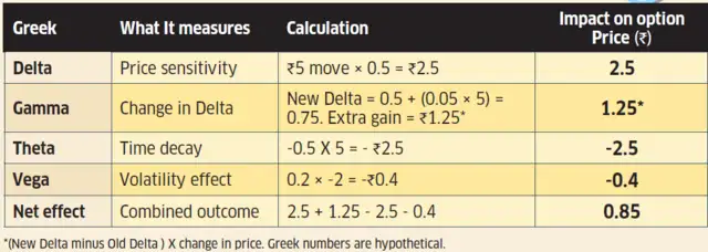
Interpretation
- Despite the stock rising Rs.5, the option gains only Rs.0.85.
- Delta and Gamma helped by increasing responsiveness to the upward move.
- But Theta eroded value steadily over 5 days.
- Vega reduced the premium further due to falling volatility.
Gamma: the accelerator
Gamma measures the rate of change of Delta for a Rs.1 move in the underlying asset. In other words, Gamma determines how fast Delta is moving. This implies that Delta is not constant and it keeps changing as the price of the underlying changes.
For retail traders, Gamma is a doubleedged sword. If your view is directionally right, Gamma works in your favour by increasing Delta and accelerating profits. If wrong, Gamma reduces Delta, slowing recovery and magnifying losses.
Example:
- A call option with Delta 0.5 gains Rs.50 when the market rises 100 points.
- As the trader is directionally correct, Gamma pushes Delta to 0.6, so the next 50-point rise adds Rs.30. Without Gamma effect, gain would be Rs.25.
- If the market falls (or if the trader is directionally wrong), Gamma shrinks Delta to 0.4.
- Next day, if market gains 50 points, call premium will now increase by Rs.20 (50 X 0.4).
- Without Gamma effect, the call premium would have gone up by Rs.25. This implies that option becomes less responsive to recovery due to Gamma effect.
Gamma and moneyness
- ATM options have high Gamma, making them highly responsive but also volatile.
- ITM options have low Gamma and are more predictable.
- OTM options have low Gamma and are largely unresponsive to Gamma effect. These options never benefit from Gamma because they expire worthless before becoming relevant.
Theta: the silent destroyer
Theta measures time decay—the amount an option loses in value each day, assuming all else remains constant. It is always negative for buyers and accelerates near expiry.
This ties back to extrinsic value—the premium traders pay for the chance that anoption becomes more profitable before expiry—which steadily erodes over time. Even if the market doesn’t move, an option loses value simply due to the passage of time. This is one of the reasons many retail traders end up losing money.
Example:
Day 1: A trader buys an ATM call option at Rs.6 with Delta 0.5 and Theta -0.5 per day.
After 5 days:
- The stock rises by Rs.2
- Gain from Delta = Rs.1 (Rs.2 × 0.5)
Time decay impact:
Theta erosion = Rs.2.5 (Rs.0.5 × 5 days)
Net option price: Rs. 6 + Rs.1 – Rs.2.5 = Rs.4.5
Net loss: Rs.1.5 (Rs.6 – Rs.4.5), despite being directionally right.
This shows options require not just direction—but speed. If the underlying asset price moves slowly, theta dominates delta and results in losses.
Theta and moneyness
- Highest for ATM options.
- Lower for ITM and far OTM (far OTM call option is the one with strike price significantly higher than current market price or spot price) options.
- Most retail traders buy ATM or slightly OTM options and expect gradual market movement.
- But these options have high Theta that creates steady erosion of value if there is slow movement in the underlying asset.
Vega: the volatility factor
Vega measures how sensitive an option’s price is to changes in implied volatility (IV). IV is the expected volatility or market’s expectation of future price variations.
- If Vega is 0.2, a 1% increase in IV raises the option price by Rs 0.2.
- Higher IV leads to higher premiums, lower IV reduces them.
Options often become expensive before major events (earnings, budget announcements, policy decisions). After the event, volatility drops as uncertainty disappears, leading to a fall in premiums. A trader may correctly predict direction but still lose money if falling volatility offsets gains.
Note: The numbers used in the examples are for explanation only and are hypothetical. Actual Greek values are mathematically derived from option pricing models, most commonly the Black–Scholes model.